
Predictive Model

Overview
To understand what makes a game successful, we trained a set of machine learning models to predict popularity, player appreciation, and their combined expression as a quadrant (e.g. high-popularity/low-appreciation). The goal was not only to classify games into outcome categories, but also to uncover which features influence those outcomes most — using interpretable techniques like SHAP to peer inside the “black box” of the model.
Problem Setup
We framed the task as a classification problem across three fronts:
- Popularity Score : Binary classification — high vs low based on the median score in the dataset.
- Appreciation Score : Binary classification — high vs low (also median split).
- Quadrant Prediction : Multiclass classification into four groups.
- High Popularity - High Appreciation
- High Popularity - Low Appreciation
- Low Popularity - High Appreciation
- Low Popularity - Low Appreciation
These categories help us understand how well a game resonates commercially and critically.
Data and Feature Engineering
After filtering for games with a valid Metacritic page, we worked with a refined dataset of around 5,000 games.
We used a combination of numeric, categorical, and one-hot encoded tag features:
- Numerical: required_age, dlc_count, year, is_indie, wishlist_backloggd, num_supported_languages, num_audio_languages, num_platforms
- Categorical (one-hot encoded): Tags/attributes across 9 game design categories: Themes & Moods, Top-Level Genres, Visuals & Viewpoint, Sub-Genres, Players, Story, Level Design, Sports, and initial/current_price_range.
Modeling Approach
We used the XGBoost classifier, a high-performance gradient boosting algorithm well-suited for tabular data. Each model was tuned using a grid search over key hyperparameters to balance learning ability and generalization. Key tuning strategies included:
- Keeping max_depth and n_estimators low (1–2 and 15–25 respectively),
- Monitoring early stopping to prevent overfitting,
- Using logloss and mlogloss as evaluation metrics.
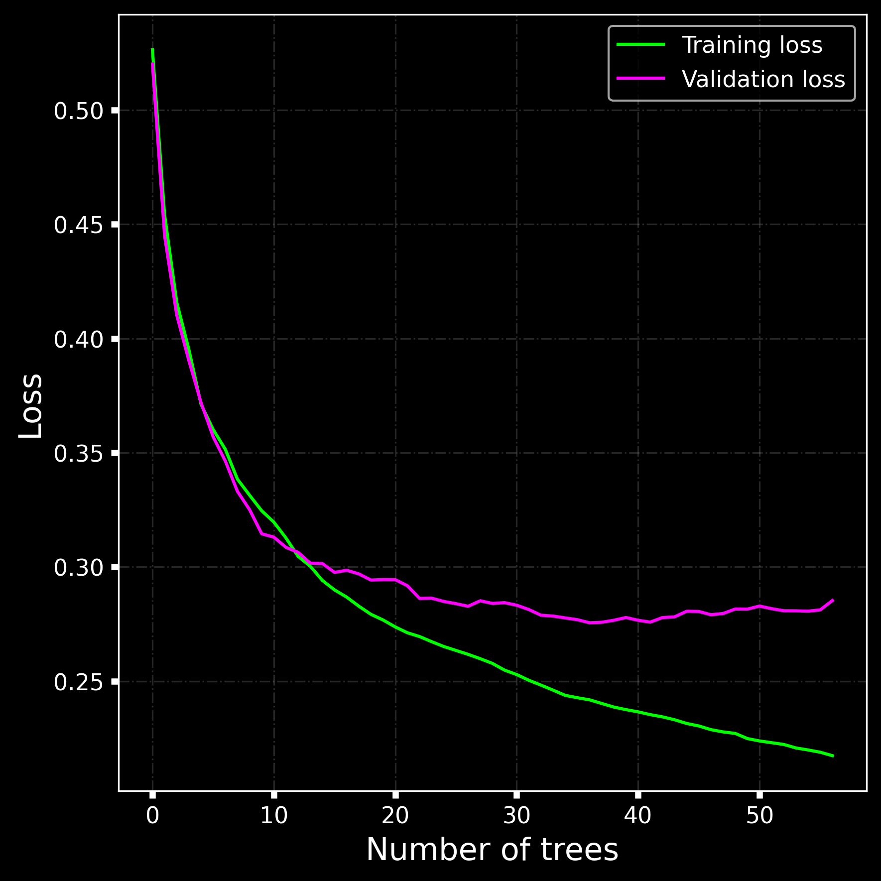
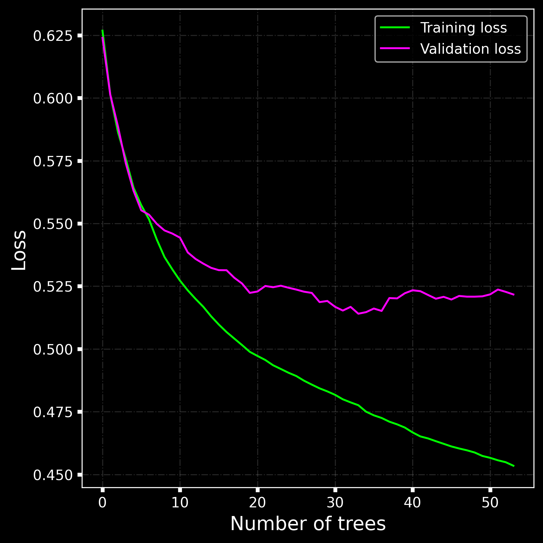
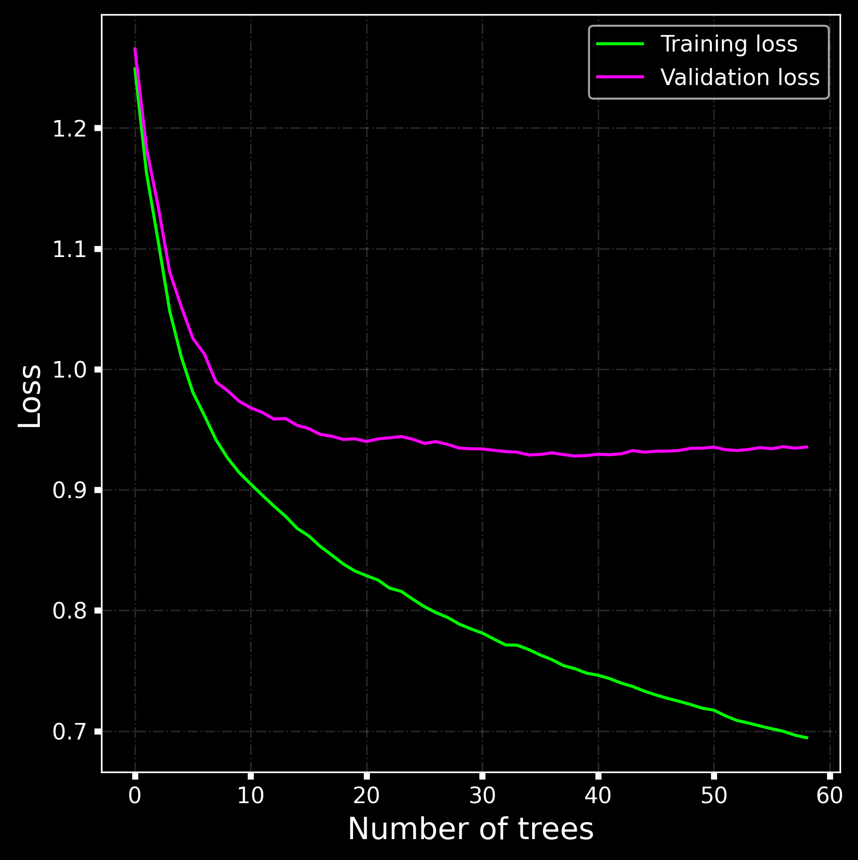
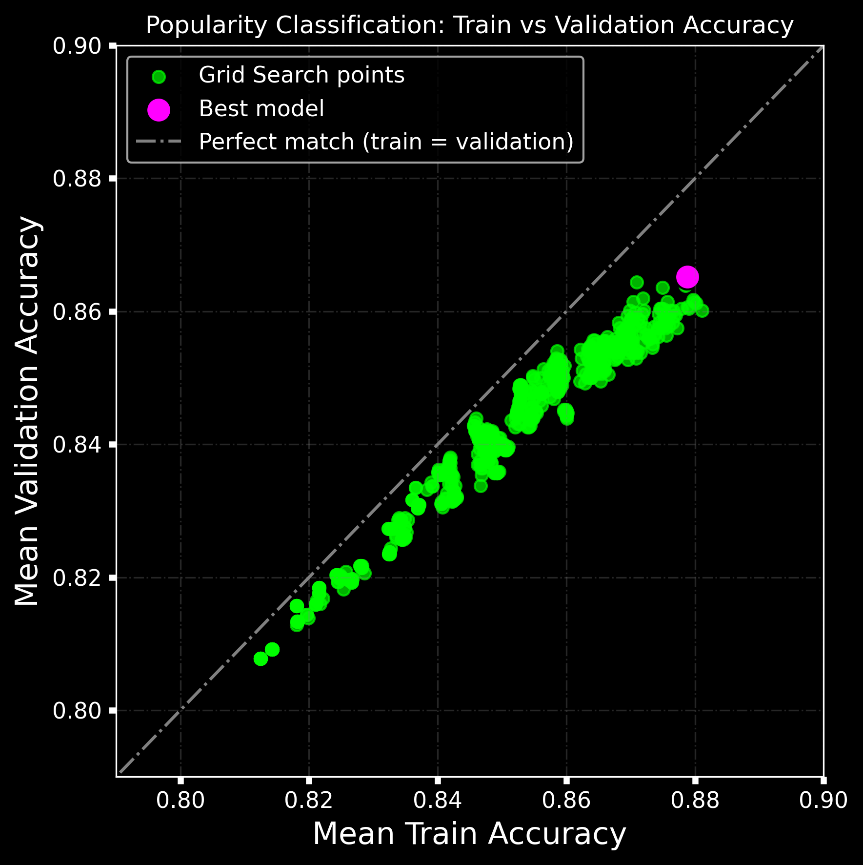
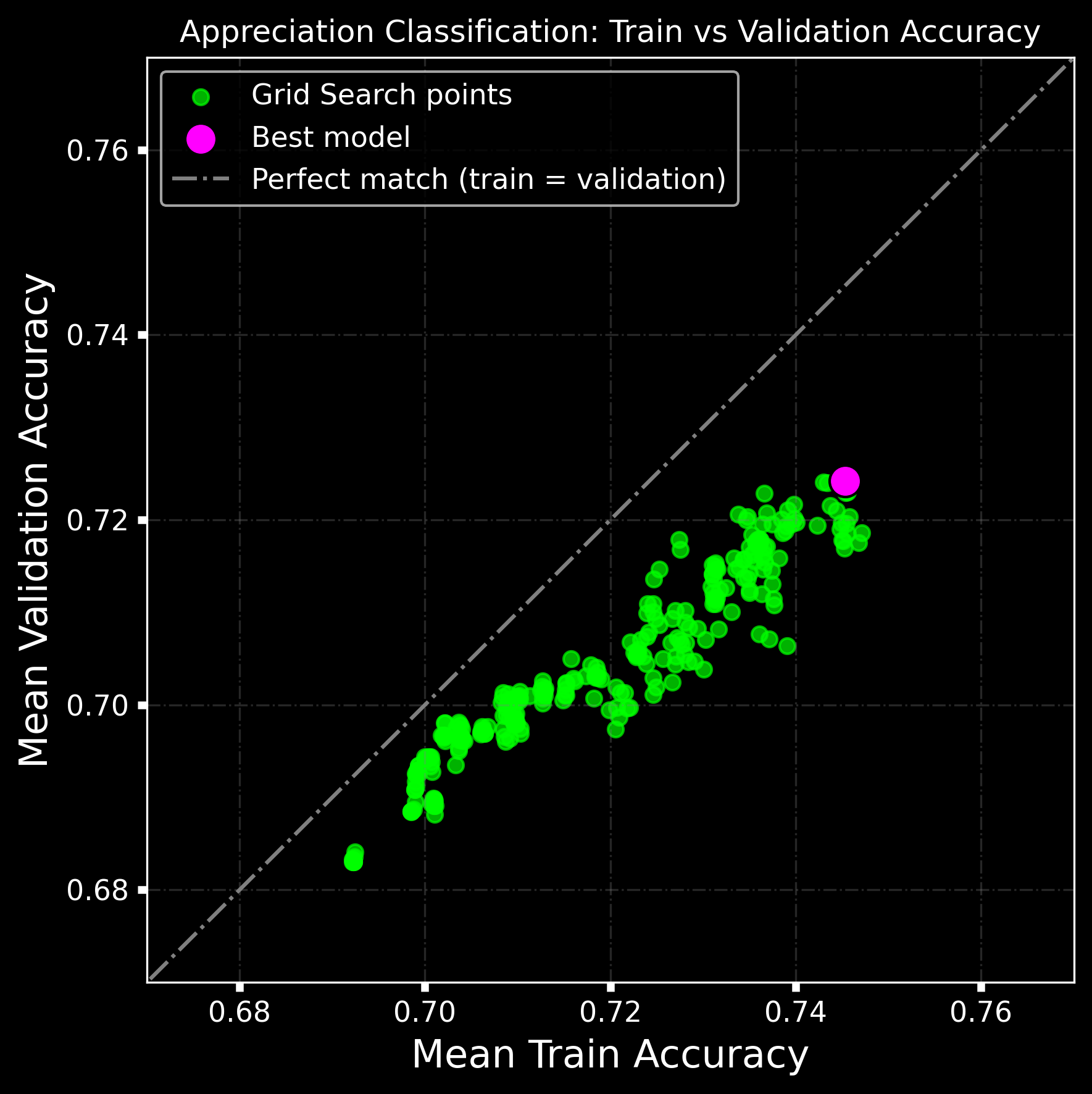
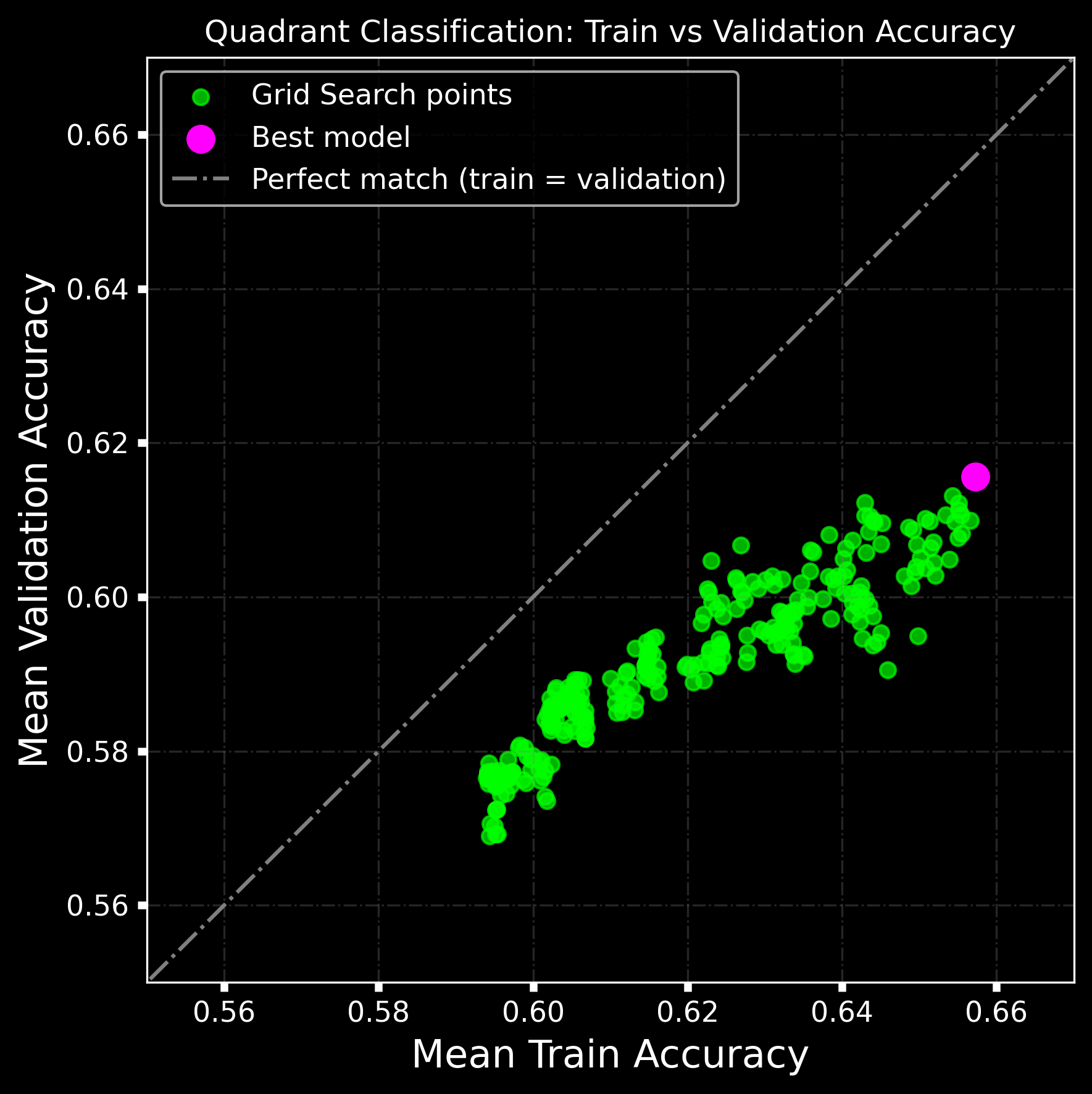
max_depth = 2. In each case, to prevent overfitting the number of estimators must be kept low. In order to find the best parameters configuration we used Gridsearch. In Fig.2 we display the best configurations with magenta dots.
Model Performance
Each of our (best) models outperforms the corresponding Dummy Classifier that would always give the most frequent class as output resulting in the following accuracy values:
- Popularity-only model: 50% (since our classes are balanced in this case)
- Appreciation-only model: 50% (since our classes are balanced in this case)
- Quadrant model: 33%
Tab.1 reports parameters and performance for our best models. Given these results we can state that our classifiers are indeed learning patterns from data.
| Model | Mean Train Accuracy (CV) | Mean Validation Accuracy (CV) | Test Accuracy | Parameters | Notes |
| Popularity Model | 0.879 | 0.865 | 0.838 | max_depth: 2, n_estimators: 25, learning_rate: 0.5, colsample_bytree: 0.8, subsample: 0.8, reg_alpha: 0.5, reg_lambda: 0.8, | Strong performance with minimal overfitting |
| Appreciation Model | 0.746 | 0.725 | 0.729 | max_depth: 2, n_estimators: 20, learning_rate: 0.5, colsample_bytree: 0.8, subsample: 0.5, reg_alpha: 0.5, reg_lambda: 1, | Predictive accuracy is solid, especially given that appreciation is inherently more subjective. |
| Quadrant Classifier | 0.657 | 0.616 | 0.611 | max_depth: 2, n_estimators: 20, learning_rate: 0.5, colsample_bytree: 0.8, subsample: 0.8, reg_alpha: 0, reg_lambda: 0.5, | Multi-class prediction is understandably more difficult, but the model performs well enough to support deeper SHAP-based analysis of what drives game outcomes. |
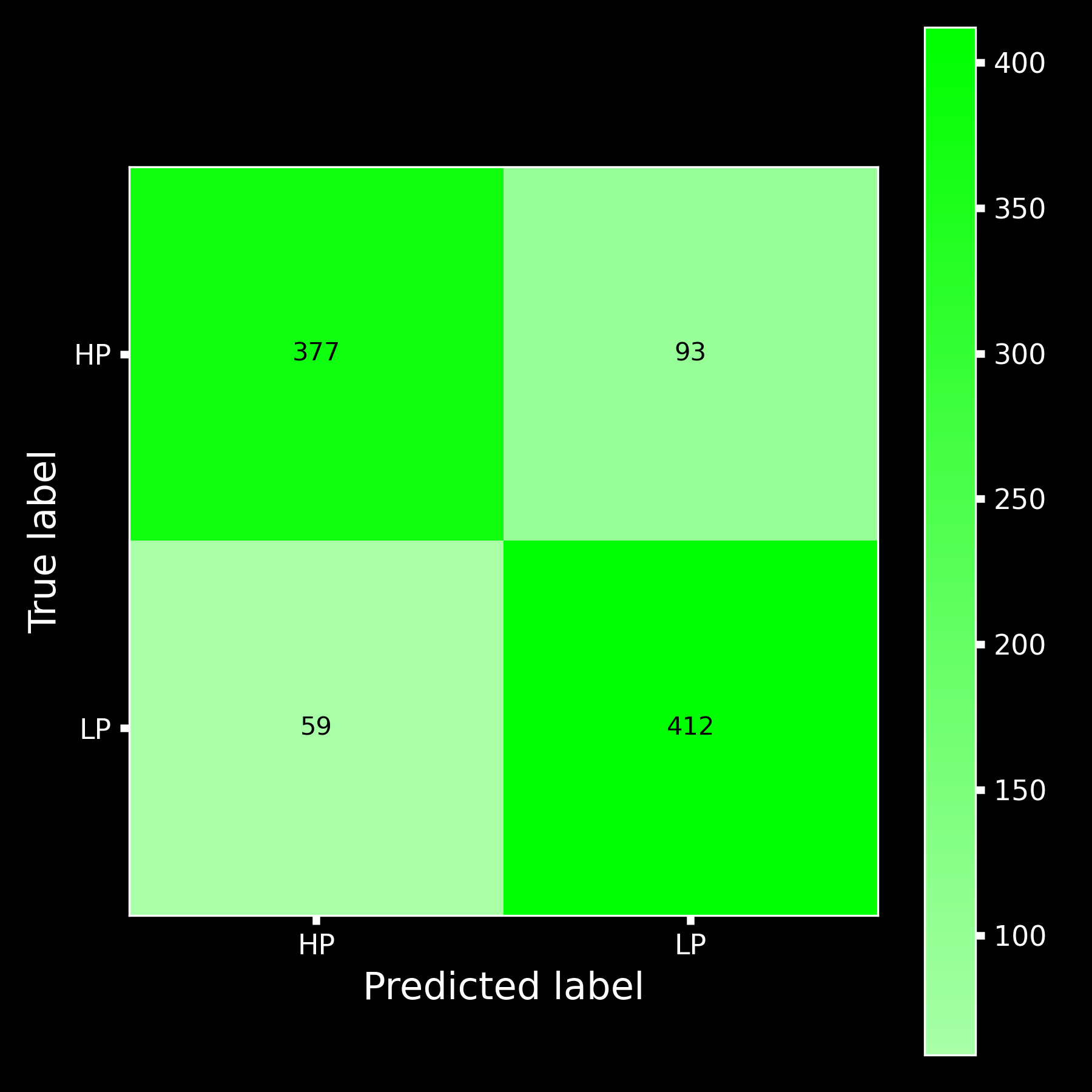
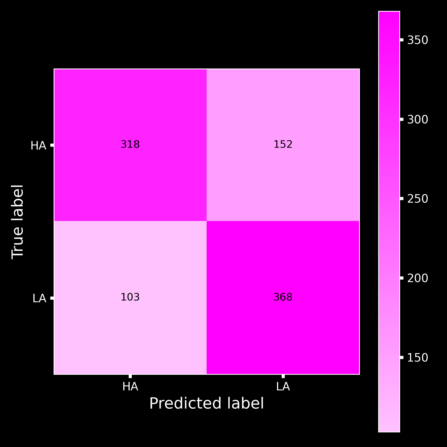
Tab.2, Tab.3 and Tab.4 show the classification reports for each model, while Fig.3 displays the corresponding confusion matrices.
| precision | recall | f1-score | support | |
| 0 | 0.816 | 0.875 | 0.844 | 471 |
| 1 | 0.865 | 0.802 | 0.832 | 470 |
| accuracy | 0.838 | 941 | ||
| macro avg | 0.840 | 0.838 | 0.838 | 941 |
| weighted avg | 0.840 | 0.838 | 0.838 | 941 |
| precision | recall | f1-score | support | |
| 0 | 0.708 | 0.781 | 0.743 | 471 |
| 1 | 0.755 | 0.677 | 0.714 | 470 |
| accuracy | 0.729 | 941 | ||
| macro avg | 0.732 | 0.729 | 0.728 | 941 |
| weighted avg | 0.732 | 0.729 | 0.728 | 941 |
| precision | recall | f1-score | support | |
| 0 | 0.709 | 0.659 | 0.683 | 311 |
| 1 | 0.483 | 0.631 | 0.547 | 160 |
| 2 | 0.410 | 0.544 | 0.468 | 160 |
| 3 | 0.788 | 0.587 | 0.673 | 310 |
| accuracy | 0.611 | 941 | ||
| macro avg | 0.598 | 0.605 | 0.593 | 941 |
| weighted avg | 0.646 | 0.611 | 0.620 | 941 |
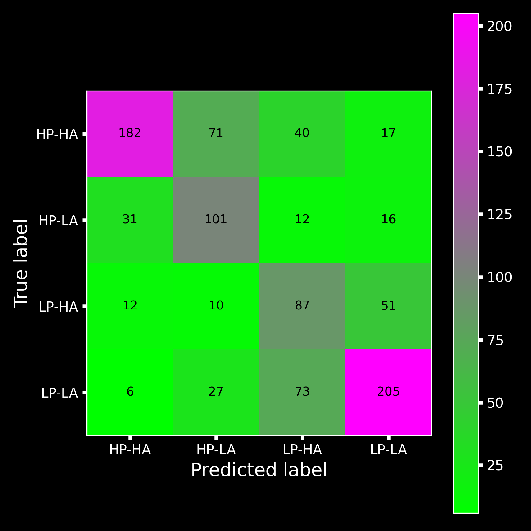
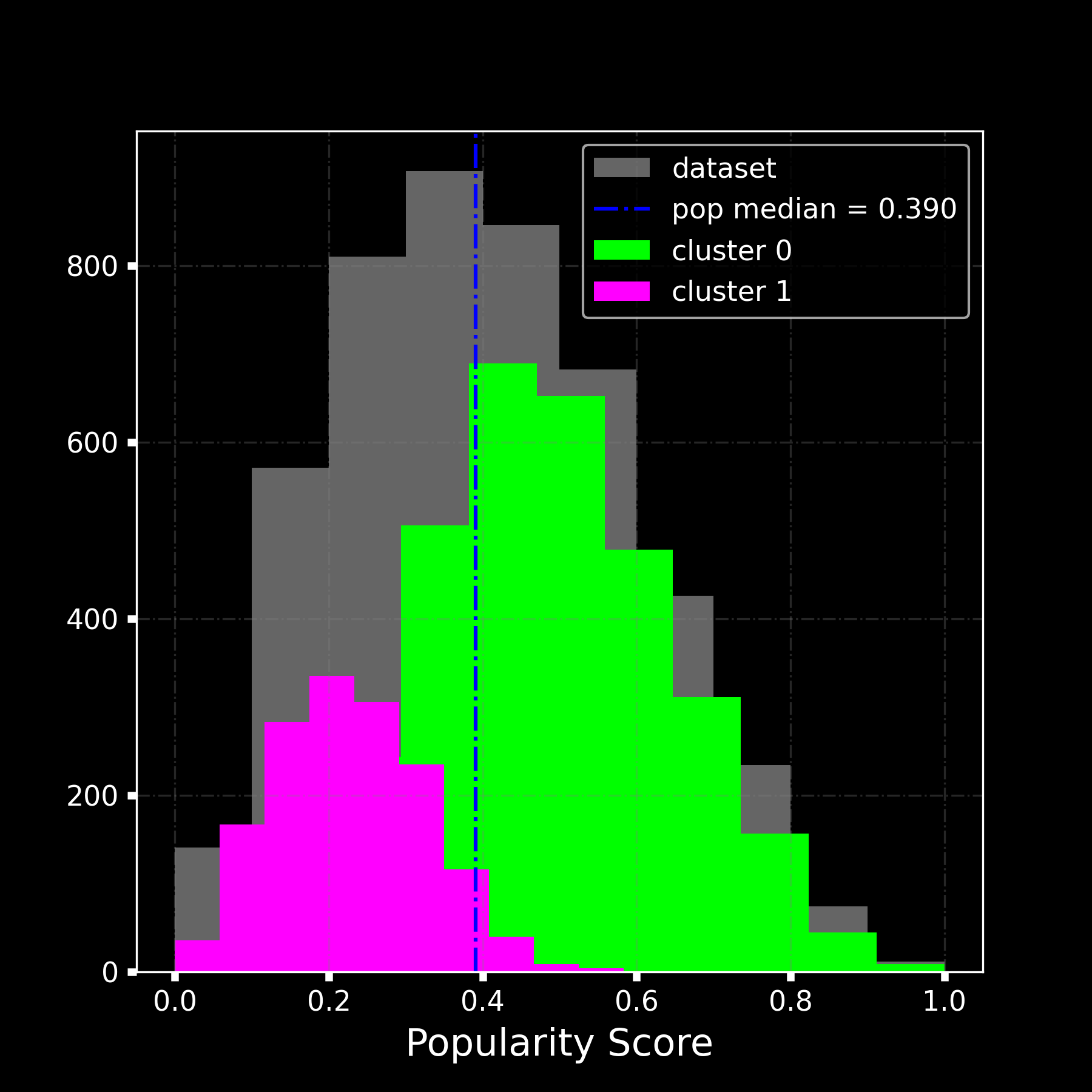
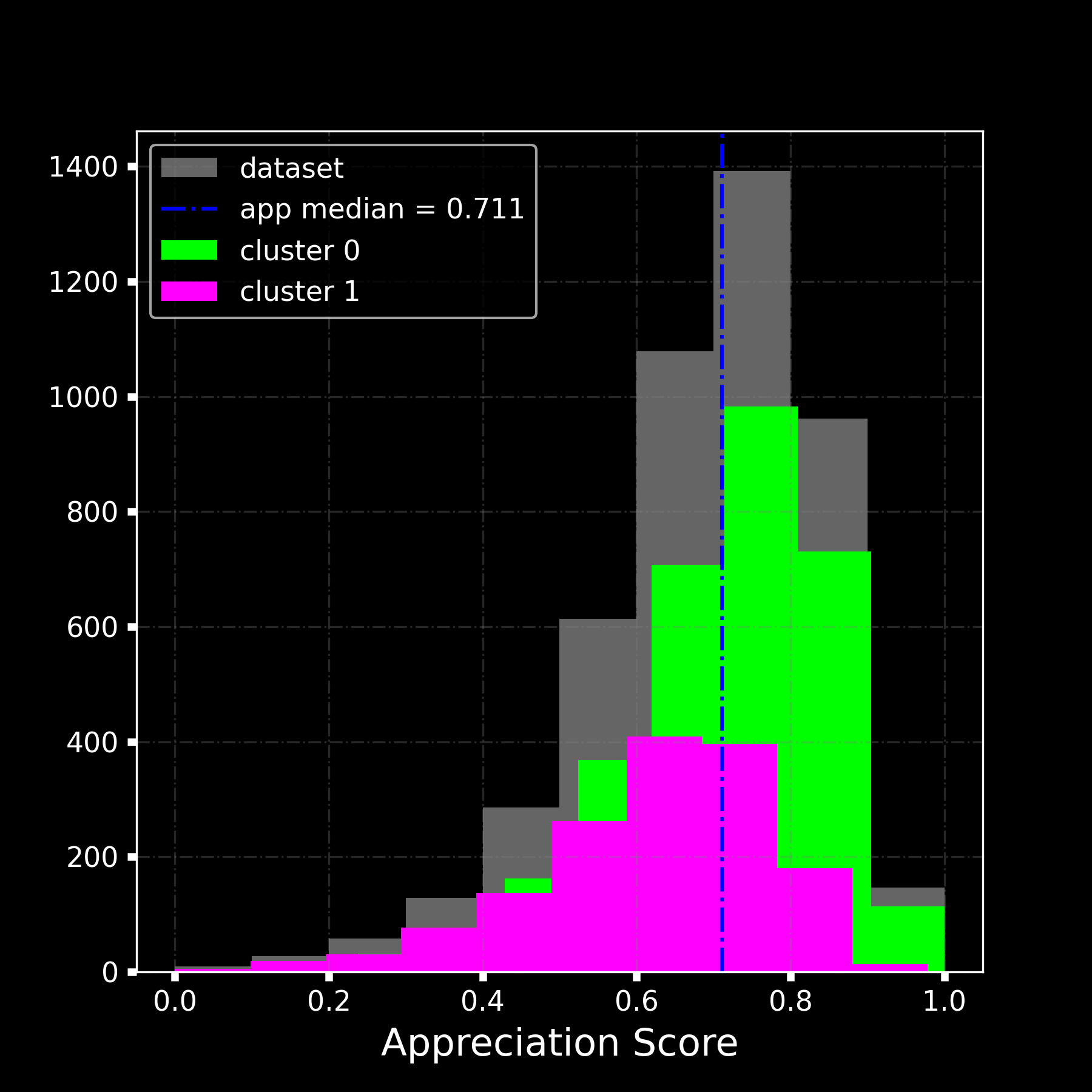
In order to have some insight on the model performances in the multiclass classification task, we ran a clustering algorithm (Kmeans) using as features the ones defining Popularity and Appreciation scores. This approach results in two macro-clusters. Fig.4 shows distributions for popularity and appreciation for each cluster. As we can see, only popularity can be considered well separated into two classes (High Popularity and Low Popularity), while it is not possible to obtain an analogous separation level for appreciation. This can justify the worse predictive performance of our multiclass model. Tab.5 reports mean and standard deviation for popularity and appreciation for the whole dataset and the two clusters.
| Mean | Std | |
| Dataset Popularity | 0.403 | 0.185 |
| Cluster 0 Popularity | 0.488 | 0.155 |
| Cluster 1 Popularity | 0.228 | 0.097 |
| Dataset Appreciation | 0.687 | 0.148 |
| Cluster 0 Appreciation | 0.719 | 0.135 |
| Cluster 1 Appreciation | 0.623 | 0.153 |
Explainability: Using SHAP
To move beyond raw accuracy and into insight, we used SHAP (SHapley Additive exPlanations) to interpret the models. SHAP provides per-feature attribution scores that show not only what features matter, but how they influence predictions, whether positively or negatively.
The SHAP summary plot shows the impact of each feature on the model’s predictions across all samples. Each dot represents a game, positioned horizontally by how much that feature pushed the prediction higher or lower (the SHAP value). The color of the dot indicates the actual value of the feature for that game — with red meaning a high value and blue a low one. Features are sorted top to bottom by their overall importance (mean absolute SHAP value), so those at the top have the greatest influence on the model’s output. This plot helps us see not only which features matter the most, but also how different values of those features affect predictions.
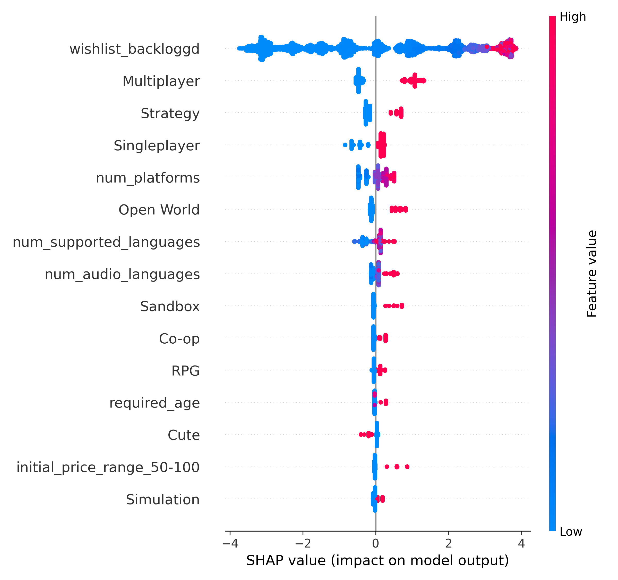
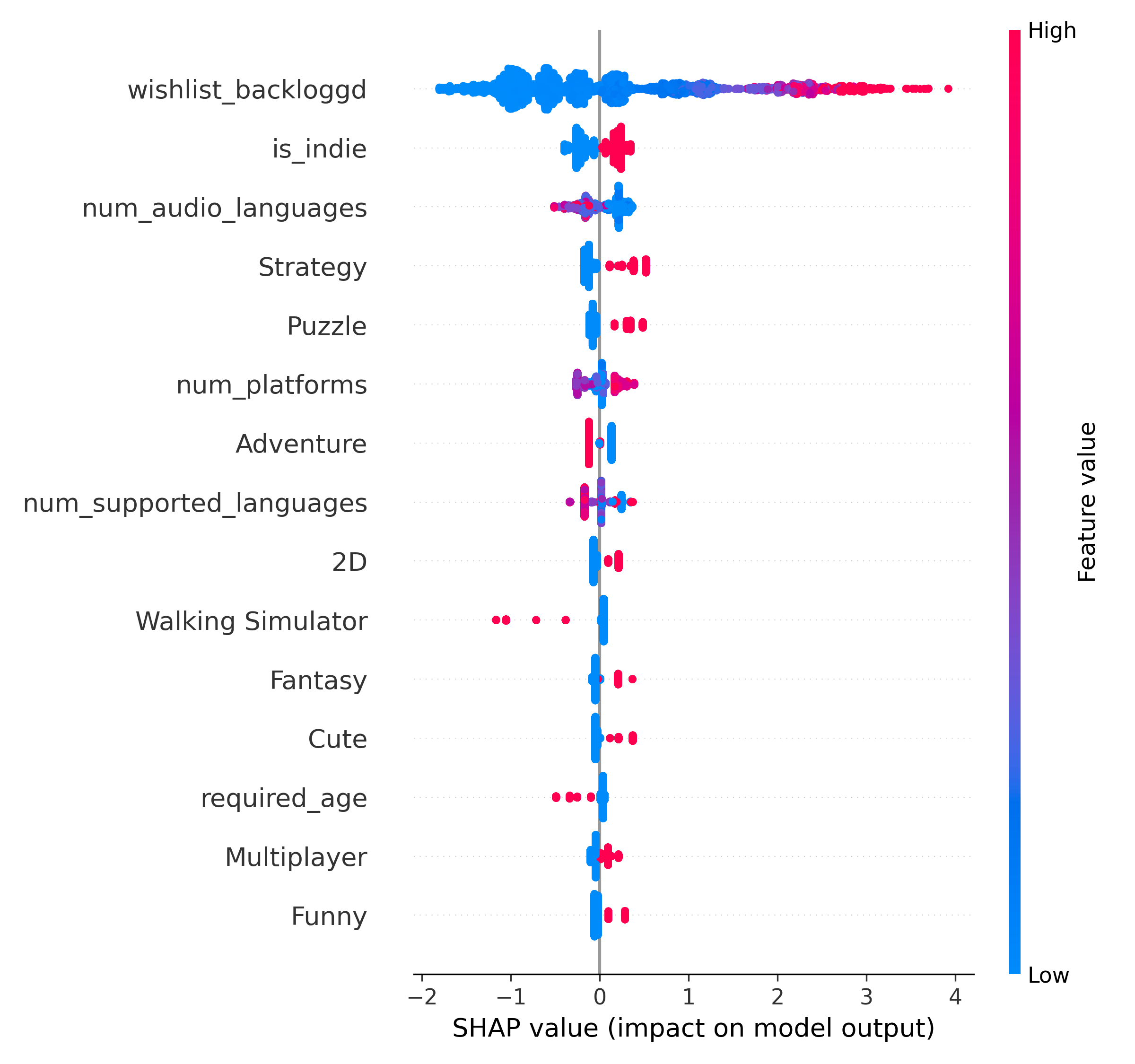
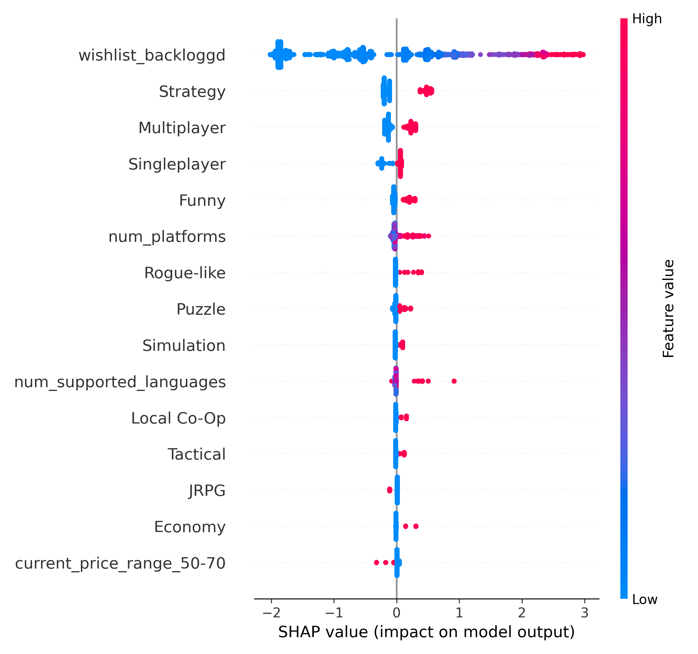
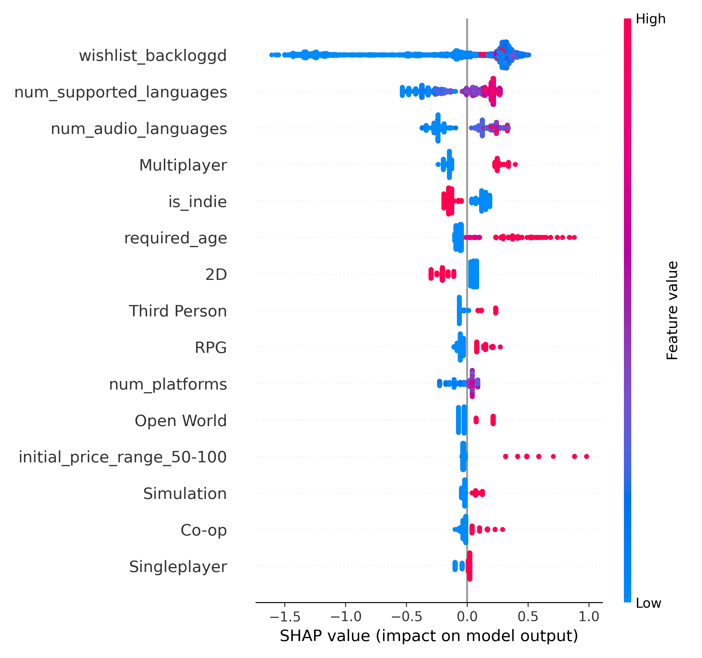
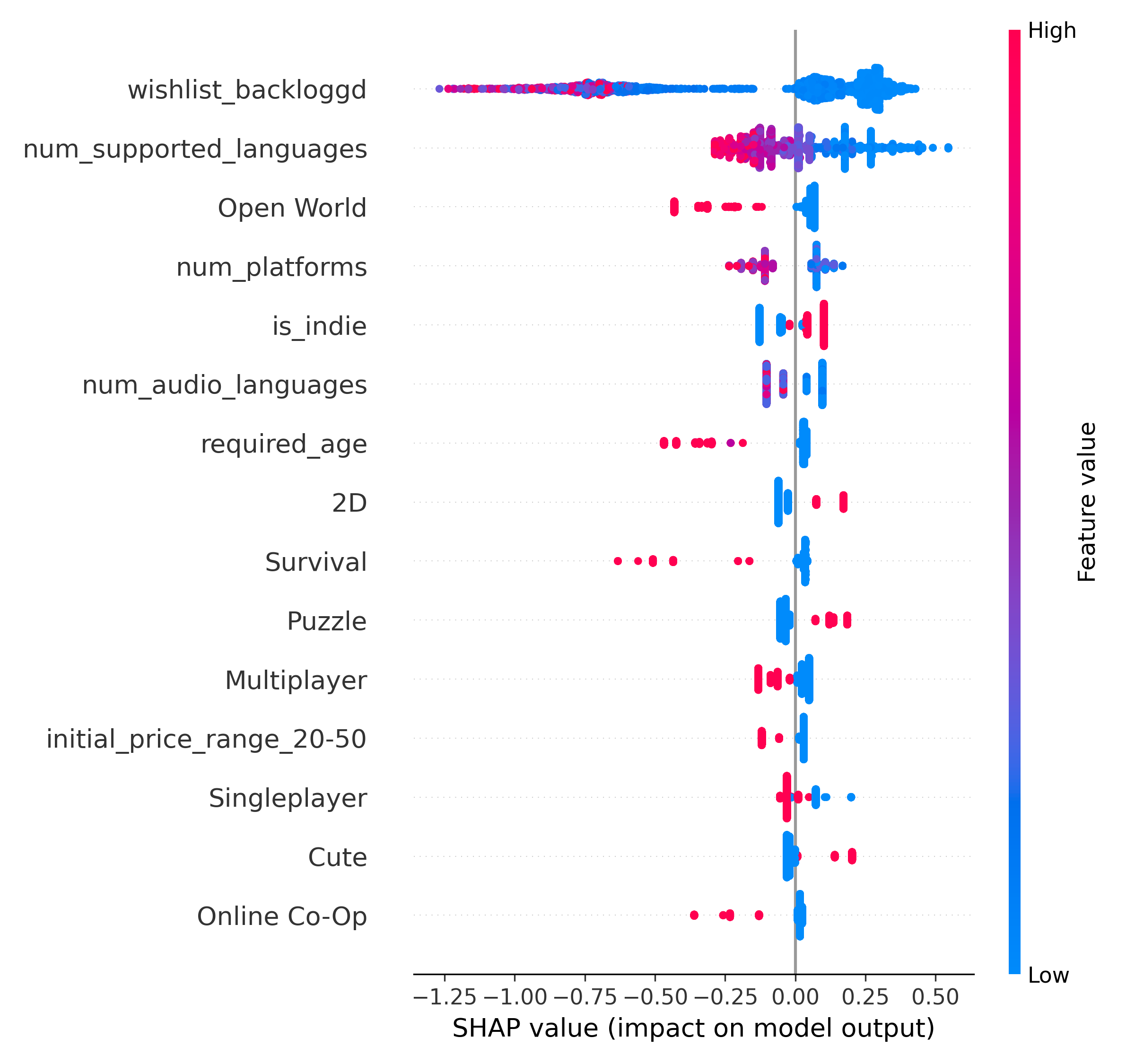
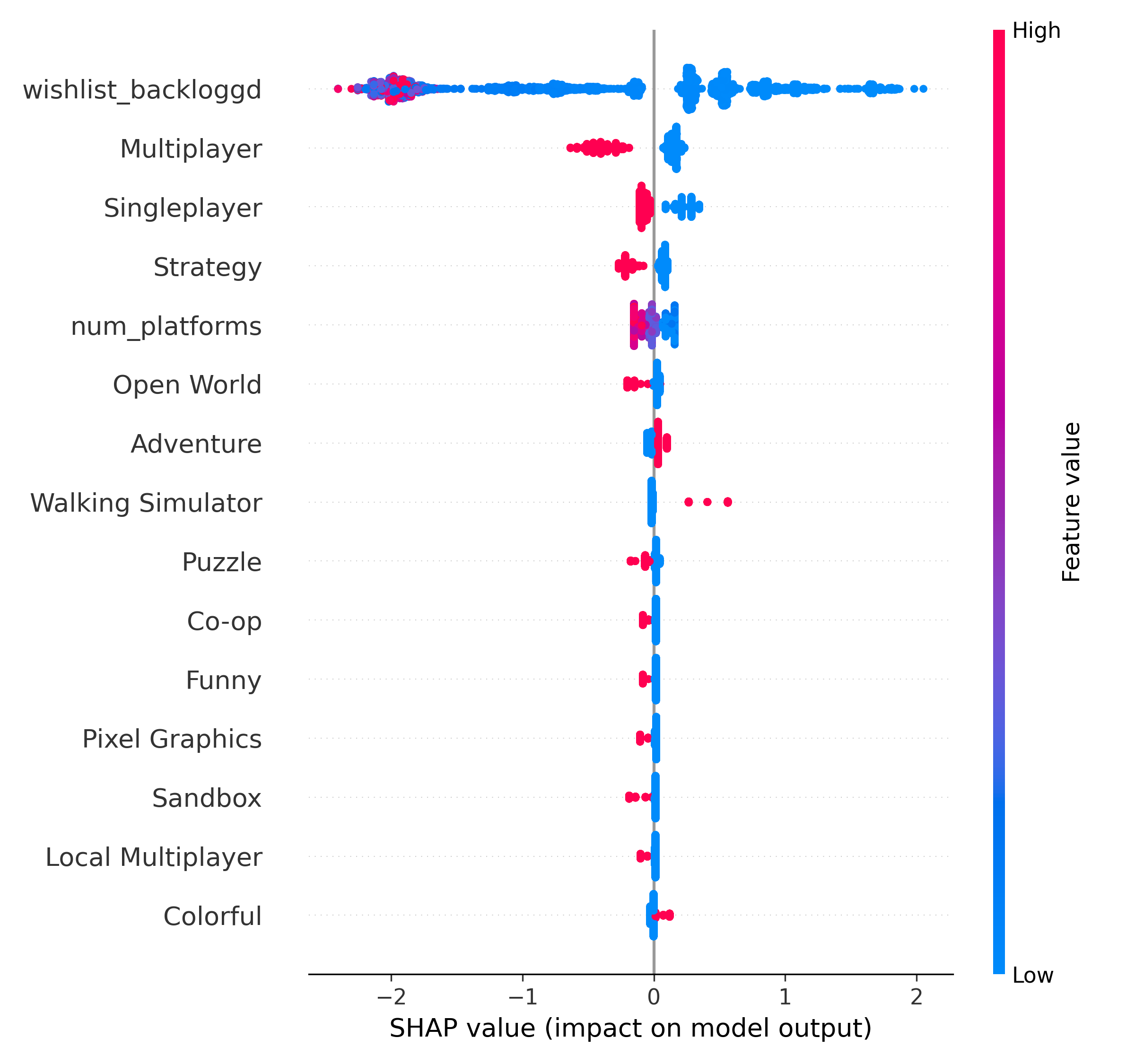
SHAP helped reveal:
- The dominant influence of wishlist_backloggd across all models;
- The asymmetric importance of features like Multiplayer, Strategy, is_indie, and Open World;
- That high appreciation often hinges on tags like Puzzle, Cute, or Funny, while popularity leans on broader features like multiplayer or platform support;
- The complexity of quadrant dynamics — e.g., how some features protect against a "low/low" outcome, while others increase the risk of being overhyped but underwhelming.
Limitations of our approach
- Data size (~5,000 games) is relatively modest, especially for deep modeling of subjective traits like appreciation;
- Tag quality depends on how consistently games are labeled, which may introduce noise;
- Temporal generalization is not tested — models were trained on a snapshot and may not fully predict future hits;
- Additional features related to marketing or reviews content could add deeper context to future models.